Project: Train a Quadcopter How to Fly
Controlling the Quadcopter
The agent controls the quadcopter by setting the revolutions per second on each of its four rotors. The provided agent in the Basic_Agent class below always selects a random action for each of the four rotors. These four speeds are returned by the act method as a list of four floating-point numbers.
import random

class Basic_Agent():
    def __init__(self, task):
        self.task = task

    def act(self):
        new_thrust = random.gauss(450., 25.)
        return [new_thrust + random.gauss(0., 1.) for x in range(4)]
The labels list below annotates statistics that are saved while running the simulation. All of this information is saved in a text file data.txt and stored in the dictionary results.
%load_ext autoreload
%autoreload 2

import csv
import numpy as np
from task import Task

# Modify the values below to give the quadcopter a different starting position.
runtime = 5.                                     # time limit of the episode
init_pose = np.array([0., 0., 10., 0., 0., 0.])  # initial pose
init_velocities = np.array([0., 0., 0.])         # initial velocities
init_angle_velocities = np.array([0., 0., 0.])   # initial angle velocities
file_output = 'data.txt'                         # file name for saved results

# Setup
task = Task(init_pose, init_velocities, init_angle_velocities, runtime)
agent = Basic_Agent(task)
done = False
labels = ['time', 'x', 'y', 'z', 'phi', 'theta', 'psi', 'x_velocity',
          'y_velocity', 'z_velocity', 'phi_velocity', 'theta_velocity',
          'psi_velocity', 'rotor_speed1', 'rotor_speed2', 'rotor_speed3', 'rotor_speed4']
results = {x : [] for x in labels}

# Run the simulation, and save the results.
with open(file_output, 'w') as csvfile:
    writer = csv.writer(csvfile)
    writer.writerow(labels)
    while True:
        rotor_speeds = agent.act()
        _, _, done = task.step(rotor_speeds)
        to_write = [task.sim.time] + list(task.sim.pose) + list(task.sim.v) + list(task.sim.angular_v) + list(rotor_speeds)
        for ii in range(len(labels)):
            results[labels[ii]].append(to_write[ii])
        writer.writerow(to_write)
        if done:
            break
import matplotlib.pyplot as plt
%matplotlib inline

plt.plot(results['time'], results['x'], label='x')
plt.plot(results['time'], results['y'], label='y')
plt.plot(results['time'], results['z'], label='z')
plt.legend()
_ = plt.ylim()

The next code cell visualizes the velocity of the quadcopter.
plt.plot(results['time'], results['x_velocity'], label='x_hat')
plt.plot(results['time'], results['y_velocity'], label='y_hat')
plt.plot(results['time'], results['z_velocity'], label='z_hat')
plt.legend()
_ = plt.ylim()

Next, you can plot the Euler angles (the rotation of the quadcopter over the $x$-, $y$-, and $z$-axes),
plt.plot(results['time'], results['phi'], label='phi')
plt.plot(results['time'], results['theta'], label='theta')
plt.plot(results['time'], results['psi'], label='psi')
plt.legend()
_ = plt.ylim()

before plotting the velocities (in radians per second) corresponding to each of the Euler angles.
plt.plot(results['time'], results['phi_velocity'], label='phi_velocity')
plt.plot(results['time'], results['theta_velocity'], label='theta_velocity')
plt.plot(results['time'], results['psi_velocity'], label='psi_velocity')
plt.legend()
_ = plt.ylim()

plt.plot(results['time'], results['rotor_speed1'], label='Rotor 1 revolutions / second')
plt.plot(results['time'], results['rotor_speed2'], label='Rotor 2 revolutions / second')
plt.plot(results['time'], results['rotor_speed3'], label='Rotor 3 revolutions / second')
plt.plot(results['time'], results['rotor_speed4'], label='Rotor 4 revolutions / second')
plt.legend()
_ = plt.ylim()

task.sim.pose(the position of the quadcopter in ($x,y,z$) dimensions and the Euler angles),task.sim.v(the velocity of the quadcopter in ($x,y,z$) dimensions), andtask.sim.angular_v(radians/second for each of the three Euler angles).
# the pose, velocity, and angular velocity of the quadcopter at the end of the episode
print(task.sim.pose)
print(task.sim.v)
print(task.sim.angular_v)
In the sample task in task.py, we use the 6-dimensional pose of the quadcopter to construct the state of the environment at each timestep.
The Task
The __init__() method is used to initialize several variables that are needed to specify the task.
- The simulator is initialized as an instance of the
PhysicsSimclass (fromphysics_sim.py). - Inspired by the methodology in the original DDPG paper, we make use of action repeats. For each timestep of the agent, we step the simulation
action_repeatstimesteps. If you are not familiar with action repeats, please read the Results section in the DDPG paper. - We set the number of elements in the state vector. For the sample task, we only work with the 6-dimensional pose information. To set the size of the state (
state_size), we must take action repeats into account. - The environment will always have a 4-dimensional action space, with one entry for each rotor (
action_size=4). You can set the minimum (action_low) and maximum (action_high) values of each entry here. - The sample task in this provided file is for the agent to reach a target position. We specify that target position as a variable.
The reset() method resets the simulator. The agent should call this method every time the episode ends. You can see an example of this in the code cell below.
The step() method is perhaps the most important. It accepts the agent's choice of action rotor_speeds, which is used to prepare the next state to pass on to the agent. Then, the reward is computed from get_reward(). The episode is considered done if the time limit has been exceeded, or the quadcopter has travelled outside of the bounds of the simulation.
The Agent
The sample agent given in agents/policy_search.py uses a very simplistic linear policy to directly compute the action vector as a dot product of the state vector and a matrix of weights. Then, it randomly perturbs the parameters by adding some Gaussian noise, to produce a different policy. Based on the average reward obtained in each episode (score), it keeps track of the best set of parameters found so far, how the score is changing, and accordingly tweaks a scaling factor to widen or tighten the noise.
import sys
import pandas as pd
from agents.policy_search import PolicySearch_Agent
from task import Task

num_episodes = 1000
target_pos = np.array([0., 0., 10.])
task = Task(target_pos=target_pos)
agent = PolicySearch_Agent(task)

for i_episode in range(1, num_episodes+1):
    state = agent.reset_episode() # start a new episode
    while True:
        action = agent.act(state)
        next_state, reward, done = task.step(action)
        agent.step(reward, done)
        state = next_state
        if done:
            print("\rEpisode = {:4d}, score = {:7.3f} (best = {:7.3f}), noise_scale = {}".format(
                i_episode, agent.score, agent.best_score, agent.noise_scale), end="")  # [debug]
            break
    sys.stdout.flush()
This agent should perform very poorly on this task. And that's where you come in!
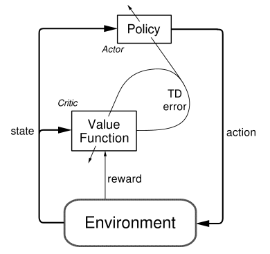
Actor-Critic Model
task.py: The task gets specified here, we will use a target position of height 10 and 0 for x and y-axes. This task can be defined as a takeoff.
import agents.agent as agent
from task import Task
import sys
import pandas as pd
#runtime = 5.                                     # time limit of the episode
num_episodes = 1000
init_pose = np.array([0., 0., 0., 0., 0., 0.])      # initial pose
init_velocities = np.array([0., 0., 0.])          # initial velocities
init_angle_velocities = np.array([0., 0., 0.])   # initial angle velocities
target_pos = np.array([0., 0., 10.])               # target => takeoff

# Setup
task = Task(init_pose, init_velocities, init_angle_velocities, runtime, target_pos)
agent = agent.DDPG(task)
done = False


pose_X = []
pose_Y = []
pose_Z = []
lastSteps = {}
steps = []
scores = []
mean_scores = []
best_scores = []
best_score = 0
last_rewards = []


for i_episode in range(1, num_episodes+1):
    state = agent.reset_episode() # start a new episode


    rewards = 0
    last_rewards = []
    while True:
        #print(agent.task.sim.__dict__["time"])
        #agent.noise.theta = agent.noise.theta*(1-i_episode/num_episodes)
        #agent.noise.sigma = agent.noise.sigma*(1-i_episode/num_episodes)
        action = agent.act(state)
        next_state, reward, done = task.step(action)
        agent.step(action, reward, next_state, done)
        rewards+=reward
        last_rewards.append(reward)
        state = next_state
        pose_X.append(task.sim.pose[0])
        pose_Y.append(task.sim.pose[1])
        pose_Z.append(task.sim.pose[2])
        lastSteps = {"X":pose_X, "Y":pose_Y, "Z":pose_Z}
        if done:
            pose_X = []
            pose_Y = []
            pose_Z = []
            scores.append(rewards)
            mean_scores.append(sum(scores)/len(scores))
            best_scores.append(best_score)
            if rewards > best_score:
                best_score = rewards
            print("\rEpisode = {:4d}, score = {:7.3f} (best = {:7.3f})".format(
                i_episode, scores[-1], best_score), end="")  # [debug]
            if i_episode % 10 == 0:
                steps.append(lastSteps)
            #assert 1==0
            break
    sys.stdout.flush()
bestSteps = steps[1]
plt.plot(range(0,len(bestSteps["X"])), bestSteps['X'], label='x')
plt.plot(range(0,len(bestSteps["X"])), bestSteps['Y'], label='y')
plt.plot(range(0,len(bestSteps["X"])), bestSteps['Z'], label='z')
plt.plot(range(0, len(last_rewards)), last_rewards, label = "Reward")
plt.legend()
Plotting the Rewards
plt.plot(range(0, len(scores)), scores, label = "Score")
plt.plot(range(0, len(scores)), mean_scores, label = "Mean Score")
plt.plot(range(0, len(scores)), best_scores, label = "Best Score")
#plt.plot(range(0, len(agent.stats["Average Score"])), agent.stats["Best Score"], label = "Best Score")
#plt.plot(range(0, len(agent.stats["Average Score"])), agent.stats["Average Score"], label = "Average Score")
plt.legend()

As you can see, the scores settle at a specific point, but this can't be considered as optimum.
Reflections
Designing the reward function
I tried different ways to make the agent learn in the specific environment for the specified task:
- using the pre-defined reward function (only comparing target position and current position)
- subtracting the standard deviation of each velocity normalized by the mean value
- combining positional aspects and velocity as stated in the article https://medium.com/@BonsaiAI/deep-reinforcement-learning-models-tips-tricks-for-writing-reward-functions-a84fe525e8e0
- I also added a reward of 5 if the agent reaches the goal at the end of an episode
- The last reward function I tried was scaling the current distance
self.sim.pose[:3]to the agent's target positionself.target_posbetween -1 and 1np.tanh(1. - 0.03* (abs(self.sim.pose[:3] - self.target_pos)).sum())
 Source: http://mathworld.wolfram.com/images/interactive/TanhReal.gif
- In addition, I created two ways to reward and penalize the agent's behavior in a more drastic way:
- If the time exceeds, the agents gets a reward of
-10.0. Due to this modification, the overall speed of the takeoff drastically changed for the better - If climbing higher than the target height, the agent receives an additional reward of
+10.0. This helped to increase the incentive to reach the overall goal
- If the time exceeds, the agents gets a reward of
My observations due to changes to the reward function:
- Even though it helped to incentify the agent to reach his goal, giving high rewards to get to the goal in a fast manner as well as even exceeding the desired height, the agent didn't learn to travel linearly on the z-axis.
- After all, this doesn't decrease the overall performance, because the learning rate and the experiences finally helped to reach the goal.
Actor-Critic Model
What learning algorithm(s) did you try? What worked best for you?
I knew, I would have to use a policy-based method. The continuous action space in which the quadcopter is moving in, doesn't leave space for value-based methods. Udacity already provided an actor critic model so I took the concept and analyzed it strengthes and weaknesses.
The combination of the underlying policy greadient method as well as the Q-value optimization provided an interesting framework to try out in the quadcopter environment.
What was your final choice of hyperparameters (such as $\alpha$, $\gamma$, $\epsilon$, etc.)?
At first, I left all the hyperparameters as they were. The results were that the agent didn't learn well enough. In consequence, I tried out different values for the following parameters:
- Gamma: I even went down to .7, but the learning curve was getting flat after a few tries
- Tau: I used the suggested .001 from the paper "Continuous Control with Deep Reinforcement Learning"
- Neural Network Architecture parameters: Detailed explanation in point 3
- Noise: I tried a linear decrease of the noise every episode, but keeping it as it was before made better results
- Replay Buffer size / batch size: 100000 & 64 -> as set before
What neural network architecture did you use (if any)? Specify layers, sizes, activation functions, etc.
For the Actor and Critic, I used two different neural network architectures. The Actor, the more simpler model is built the following:
- Dense layer with 400 neurons
- Dense layer with 300 neurons
- Relu-Activation
- In the end, the model is constructed to use the action gradients from the Critic Model to train its own weights. This is the main idea of the Actor Critic Model
- The optimizer used is the Adam optimizer, set with a learning rate of 0.0001 which has been suggested by the paper
"Continuous Control with Deep Reinforcement Learning"
- Also, dropout layers (20% dropout) and batch normalization was added to reduce overfitting
The Critic model is made up differently - mainly because this is the model to calculate Q values dependent on states AND actions whereas the Actor only takes states as inputs. The architecture looks like the following (remember: we have actions and states as input):
- Input: states
    - Dense layer with 400 neurons
    - Dense layer with 300 neurons
    - Relu-Activation

- Input: actions
    - Dense layer with 400 neurons
    - Dense layer with 300 neurons
    - Relu-Activation

- Adding up the layers:
    - Dense layer for combines actions and states
    - tanh-Activation (suggested by the paper)
    - l2 regularizer (suggested by the paper)

- The optimizer used is the Adam optimizer, set with a learning rate of 0.001 which has been suggested by the paper
"Continuous Control with Deep Reinforcement Learning"
- Like the Agent's network, the Critic's network also adopted Dropout layers and batch normalization
after each Dense layer.
As I said before, the gradients calculated by the Critic model are used to backpropagate the policy gradients to find out the optimal policy for each state.
Experiences
Was there a gradual learning curve, or an aha moment?
After all, the change oof parameters always changes the performance somehow. Especially, changing the reward function. The reward function is the key for a successful learning rate. After trying different methods to normalize and to incentify right behavior correctly, I noticed a drastic change in the learning curve of the agent. At first, it seemed random, but after applying different incentives, the performance increased in a satisfying manner.
How good was the final performance of the agent? (e.g. mean rewards over the last 10 episodes)
As I said before, the final performance was good enough to reach the goal that was set for the agent, but against my thoughts, the agent didn't learn to keep a straight route towards the target. For further improvement, you could also penalize a high variance for the euler angles.
What was the hardest part of the project? (e.g. getting started, plotting, specifying the task, etc.)
There were different stagest which had their difficulties overall:
- At first, it was hard to get an overview of the different physical metrics the agent has to deal with. I wasn't quite sure which of these variable has the greatest impact on the task I wanted to teach my agent.
- Secondly, I worked myself into the code that was provided for the Actor-Critic-Model. The combination of two neural nets of the Actor and the Critic and the use of Keras' backend function didn't seem trivial to me. Once I got the idea, I was quite impressed about it and could connect it to the lectures heard before.
- Finally, finding the critical hyperparameters and the best reward function was quite a complicated task to deal with. In the end, combining a few aspects for either two, made a quick change in behavior of the agent. And again, setting the reward function well enough, was the greatest way of increasing the agent's performance.
Did you find anything interesting in how the quadcopter or your agent behaved?
- The interesting part actually was that the the learning curve was bad after all. Checking all the parameters I was convinced that this concepts would work in the environment. Even in later episodes I thought that the already learned experience ofthe agent would help to get better results.