Deep Text Classification

Our mission

The mission is to automate job applications for everybody.

Pre-done work

I already did the following steps:

1. Crawling all the links pointing on sites that show job offers
2. Scraping each job offer with all information available
   • Job name
   • Company and link to its description site
   • Job type (part-time/full-time/freelance etc.)
   • Description (Stepstone uses html-parts to divide each section of the job offer)
3. Saving all of the divided descriptions in a DataFrame (pandas)
   • 1st column: headline
   • 2nd column: text
4. Cleaning the data
   • Reducing the labels from about 5000 to 5 so that we have the following labels:
     • company: a description of the company ("About us"-page)
     • tasks: a description of the job offered (especially the tasks of the job)
     • profile: a description of the skills needed to fulfill the job's requirements ("Your profile")
     • offer: a description of what the company offers for the applicant ("What to expect", "What we offer to you")
     • contact: contact details for the applicant (also including a hint whom to adress in the application)
5. Preprocessing Pipeline
   • In another notebook described in detail, I found a way to preprocess text data in different formats/hierarchies. Also, there are many different types of pipelines that can evolve by combining different techniques.
6. NOW: Deep Text Classification
   • We have already tried conventional Machine Learning algorithms to be able to predict job offer categories
   • Now, we want to try newer Deep Learning techniques to reach a higher accuracy.

What this notebook covers

In this notebook, the goal is to perform better than the benchmark we set with the Stochastic Gradient Descent algorithm. The result was about 95 % for the testing dataset. We will now implement a neural network to perform the same task to hopefully reach an even better accuracy.

The data we use

We use a dataframe which I scraped from www.stepstone.de. The scraping process is in a separate jupyter notebook.

Making imports

At first, we need to import the libraries and tools we need to start.

import json
import keras
from sklearn.feature_extraction.text import TfidfVectorizer 

Importing the preprocessed documents

Before we use the neural network to actually classify the data, we need to turn the documents in a vector form - which we already did in previous notebooks. So instead of having raw text data, we use the following Preprocessing Pipeline guided by the Library I created for these tasks:

Level 1

• UnicodeCleaner: Clean up messy text data with unicode characters.
• RemoveUmlauts: German umlauts like "ä", "ö", "ü" or "ß" get properly replaced
• RemoveAbbreviations: Abbreviations that might be in the way of the tokenizer (to correctly distinguish between sentences) get removed completely
• ExpandCompoundToken: Hyphen-seperated words get replaced with either both words at once or chained together
• RemoveGermanChainWords: this does the same thing as above but rather handles more complex grammatical rules to chain specific phrases together

Level 2

• Tokenization: This does the job of correctly separating words in order to work better with text

X = []
y = []

with open('preprocessed.json', 'r') as outfile:
    X = json.load(outfile)
with open('labels.json', 'r') as outfile:
    y = json.load(outfile)
X = json.loads(X)
y = json.loads(y)

Helper function for plotting the results

To be able to follow up with the progress, the neural network does, we define two plots, showing us the accuracies on the one hand, and the losses on the other hand, both for the training and testing set.

import matplotlib.pyplot as plt
plt.style.use('ggplot')

def plot_history(history):
    acc = history.history['acc']
    val_acc = history.history['val_acc']
    loss = history.history['loss']
    val_loss = history.history['val_loss']
    x = range(1, len(acc) + 1)

    plt.figure(figsize=(12, 5))
    plt.subplot(1, 2, 1)
    plt.plot(x, acc, 'b', label='Training acc')
    plt.plot(x, val_acc, 'r', label='Validation acc')
    plt.title('Training and validation accuracy')
    plt.legend()
    plt.subplot(1, 2, 2)
    plt.plot(x, loss, 'b', label='Training loss')
    plt.plot(x, val_loss, 'r', label='Validation loss')
    plt.title('Training and validation loss')
    plt.legend()

The Deep Learning class

I created a class that is supposed to be able to take vectorized text data and their labels as input. Creating an object of this class directly builds a model and displays its summary. That way, you are directly aware about how many parameters the network is going to train.

There are three important functions:

1. fitModel
   • This method provides the actual training of the neural network.
   • I used ModelCheckpoint as callback to save the best model right when an epoch is over
   • epochs is set to 5 by default. After a few iterations, I noticed that the network increased its training accuracy, but overfitting led to worse results in the validation set.
   • Saving the history of each epoch, and plotting it in the end, shows us how the network's accuracy developed during training time.
     
     

2. encoding

   • This method is there to provide correct labels to work with.

   • It makes a one-hot-encoded vector out of text labels

     

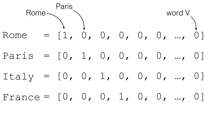
     Source: https://cdn-images-1.medium.com/max/1200/1*YEJf9BQQh0ma1ECs6x_7yQ.png
     
     

3. vectorize
   • This is the function to vectorize the text into tfidf-format
   • In previous notebooks, I already described the idea behind tfidf, but if you wish to read further information about it, I can recommend the Wikipedia article about that topic: https://en.wikipedia.org/wiki/Tf%E2%80%93idf

class DeepLearningModel():
    def __init__(self, X, y):
        from keras.models import Sequential
        from keras import layers
        from keras.layers import Dropout
        from sklearn.model_selection import train_test_split
        
        self.X_train, self.X_test, self.y_train, self.y_test = train_test_split(
                                                    self.vectorize(X), self.encoding(y), test_size=0.25, random_state=1000)
        input_dim = self.X_train.shape[1]
        model = Sequential()
        model.add(layers.Dense(256, input_dim=input_dim, activation='relu'))
        model.add(Dropout(0.2))
        model.add(layers.Dense(128, activation='relu'))
        model.add(Dropout(0.2))
        model.add(layers.Dense(5, activation='sigmoid'))
        model.compile(loss='binary_crossentropy', 
                       optimizer='adam', 
                       metrics=['accuracy'])
        self.model = model
        self.model.summary()
    
    def fitModel(self, epochs = 5):
        from keras.callbacks import ModelCheckpoint
        checkpoint = ModelCheckpoint("model.ks", monitor='val_loss', verbose=1, save_best_only=True, save_weights_only=False, mode='auto', period=1)
        history = self.model.fit(x=self.X_train, y=self.y_train, batch_size=None, epochs=epochs, verbose=1, callbacks=[checkpoint], validation_split=None, validation_data=(self.X_test, self.y_test), shuffle=True, class_weight=None, sample_weight=None, initial_epoch=0, steps_per_epoch=None, validation_steps=None)
        plot_history(history)
        
    def encoding(self, y):
        # company = 1, tasks = 5, profile = 4, offer = 3, contact = 2
        from sklearn.preprocessing import LabelEncoder
        encoder = LabelEncoder()
        y_encoded = encoder.fit_transform(y)

        from sklearn.preprocessing import OneHotEncoder
        encoder2 = OneHotEncoder(sparse=False)
        y_encoded = y_encoded.reshape(len(y_encoded), 1)
        y_encoded = encoder2.fit_transform(y_encoded)
        return y_encoded
    
    def vectorize(self, X):
        vectorizer = TfidfVectorizer(tokenizer = lambda x: x, preprocessor = lambda x: x)
        return vectorizer.fit_transform(X)

The Deep Learning Model

The architecture

The architecture is structured as follows:

1. Dense layer

   • 256 nodes (iteratively tested from 1024)
   • vectorized text as input (dimensionality of one document goes up to 126,741 in our case)

   • ReLu-activation

     

     Source: https://www.researchgate.net/profile/Leo_Pauly/publication/319235847/figure/fig3/AS:537056121634820@1505055565670/ReLU-activation-function.png

     This activation function helps to get rid of negative values and leaves positives as they are. The biggest advantage of ReLu is indeed non-saturation of its gradient, which greatly accelerates the convergence of stochastic gradient descent compared to the sigmoid / tanh functions (paper by Krizhevsky et al). In addition, it is computationally more effective than activation functions like softmax or sigmoid.
     
     

2. Dense layer

   • 128 nodes (iteratively tested from 512)
   • it takes the input from the layer before
   • ReLu ativation (picture above)

1. Dropout layers in between

   • These dropout layers with a dropout of 20 %

     

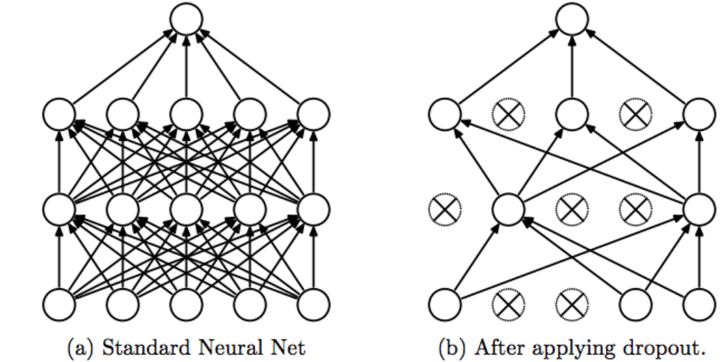
     Source: https://cdn-images-1.medium.com/max/1200/1*iWQzxhVlvadk6VAJjsgXgg.png

     These layers help to reduce overfitting. Because 20% of the randomly defined nodes are not participating in learning, other nodes are better trained. "A fully connected layer occupies most of the parameters, and hence, neurons develop co-dependency amongst each other during training which curbs the individual power of each neuron leading to over-fitting of training data." (https://medium.com/@amarbudhiraja/https-medium-com-amarbudhiraja-learning-less-to-learn-better-dropout-in-deep-machine-learning-74334da4bfc5)
     
     

1. Dense Output layer

   • 5 nodes (that represent each text category)

   • sigmoid activation

     

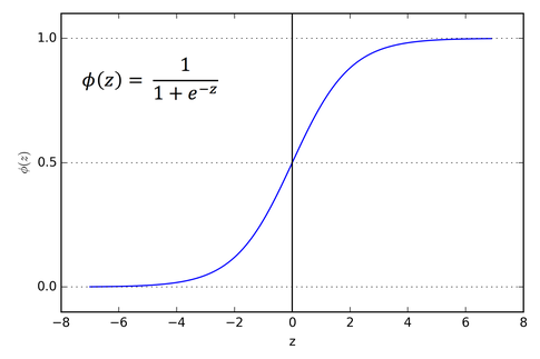
     Source: https://cdn-images-1.medium.com/max/1600/1*Xu7B5y9gp0iL5ooBj7LtWw.png

     This activation function is used to assure that the output data is scaled between 0 and 1. This means, that each of the category gets assigned a percentage value indicating how likely a text is represented by each category.
     
     

2. Adam Optimizer

   • The Adam optimizer is the most popular optimizer for Deep Learning

   • The method is straightforward to implement, is computationally efficient, has little memory requirements, is invariant to diagonal rescaling of the gradients, and is well suited for problems that are large in terms of data and/or parameters (https://arxiv.org/pdf/1412.6980.pdf)

     

     Source: https://3qeqpr26caki16dnhd19sv6by6v-wpengine.netdna-ssl.com/wp-content/uploads/2017/05/Comparison-of-Adam-to-Other-Optimization-Algorithms-Training-a-Multilayer-Perceptron.png

     Further information: https://arxiv.org/pdf/1412.6980.pdf
     
     

Here's the whole architecture in one view:

Please note: I didn't use all the nodes that are created within the net. This is because there's no proper way to display all the input nodes (126,741) and the other ones. This image only gives you an idea about how the nodes are connected to each other and how the input is transformed into an output.

dl = DeepLearningModel(X,y)

_________________________________________________________________
Layer (type)                 Output Shape              Param #   
=================================================================
dense_4 (Dense)              (None, 256)               32445952  
_________________________________________________________________
dropout_3 (Dropout)          (None, 256)               0         
_________________________________________________________________
dense_5 (Dense)              (None, 128)               32896     
_________________________________________________________________
dropout_4 (Dropout)          (None, 128)               0         
_________________________________________________________________
dense_6 (Dense)              (None, 5)                 645       
=================================================================
Total params: 32,479,493
Trainable params: 32,479,493
Non-trainable params: 0
_________________________________________________________________

C:\Users\Thorben\Documents\workspace\GPU_Environment\lib\site-packages\sklearn\preprocessing\_encoders.py:368: FutureWarning: The handling of integer data will change in version 0.22. Currently, the categories are determined based on the range [0, max(values)], while in the future they will be determined based on the unique values.
If you want the future behaviour and silence this warning, you can specify "categories='auto'".
In case you used a LabelEncoder before this OneHotEncoder to convert the categories to integers, then you can now use the OneHotEncoder directly.
  warnings.warn(msg, FutureWarning)

dl.fitModel()

Train on 32661 samples, validate on 10888 samples
Epoch 1/5
32661/32661 [==============================] - 54s 2ms/step - loss: 0.1160 - acc: 0.9636 - val_loss: 0.0718 - val_acc: 0.9794

Epoch 00001: val_loss improved from inf to 0.07183, saving model to model.ks
Epoch 2/5
32661/32661 [==============================] - 53s 2ms/step - loss: 0.0289 - acc: 0.9913 - val_loss: 0.0792 - val_acc: 0.9788

Epoch 00002: val_loss did not improve from 0.07183
Epoch 3/5
32661/32661 [==============================] - 52s 2ms/step - loss: 0.0079 - acc: 0.9976 - val_loss: 0.0958 - val_acc: 0.9782

Epoch 00003: val_loss did not improve from 0.07183
Epoch 4/5
32661/32661 [==============================] - 53s 2ms/step - loss: 0.0047 - acc: 0.9985 - val_loss: 0.1033 - val_acc: 0.9784

Epoch 00004: val_loss did not improve from 0.07183
Epoch 5/5
32661/32661 [==============================] - 53s 2ms/step - loss: 0.0037 - acc: 0.9988 - val_loss: 0.1108 - val_acc: 0.9783

Epoch 00005: val_loss did not improve from 0.07183

Conclusion

As you can see, the training accuracy rises to about 0.998 which is a very good accuracy. But, we have to take an even closer look at the validation accuracy, which stays at an even level but has highest numbers in the first epoch.

The losses show the same picture, whereas this gives us more confidence in trusting the earliest epoch. After all, we could even train the net for one epoch, which gives us a very satisfying accuracy value of nearly 98 %.